Data Analytics • Healthcare
Breast Cancer Diagnosis Dashboard
Built with Tableau using Kaggle’s Breast Cancer Wisconsin (Diagnostic) dataset.
30
Cell features explored
2
Diagnosis groups
4
Dashboard views
Dashboard Preview
Each sample in the dataset is described by 30 features of cell nuclei, measuring size, shape, smoothness, and texture. For example, malignant tumors often have larger radii, irregular edges (high concavity), and higher complexity (fractal dimension). These measurements allow us to distinguish between benign and malignant tumors.
- Benign tumors usually have small, smooth, symmetric nuclei with low concavity.
- Malignant tumors often show large, irregular, jagged nuclei with high concavity and complex edges.
Tools & Technologies
- Tableau Public (interactive analytics & dashboarding)
- Python (pandas) / Google Colab for correlation prep
- SQL (PostgreSQL) for table schema & EDA queries (optional)
- VS Code for project packaging & GitHub publishing
Dashboard Pages
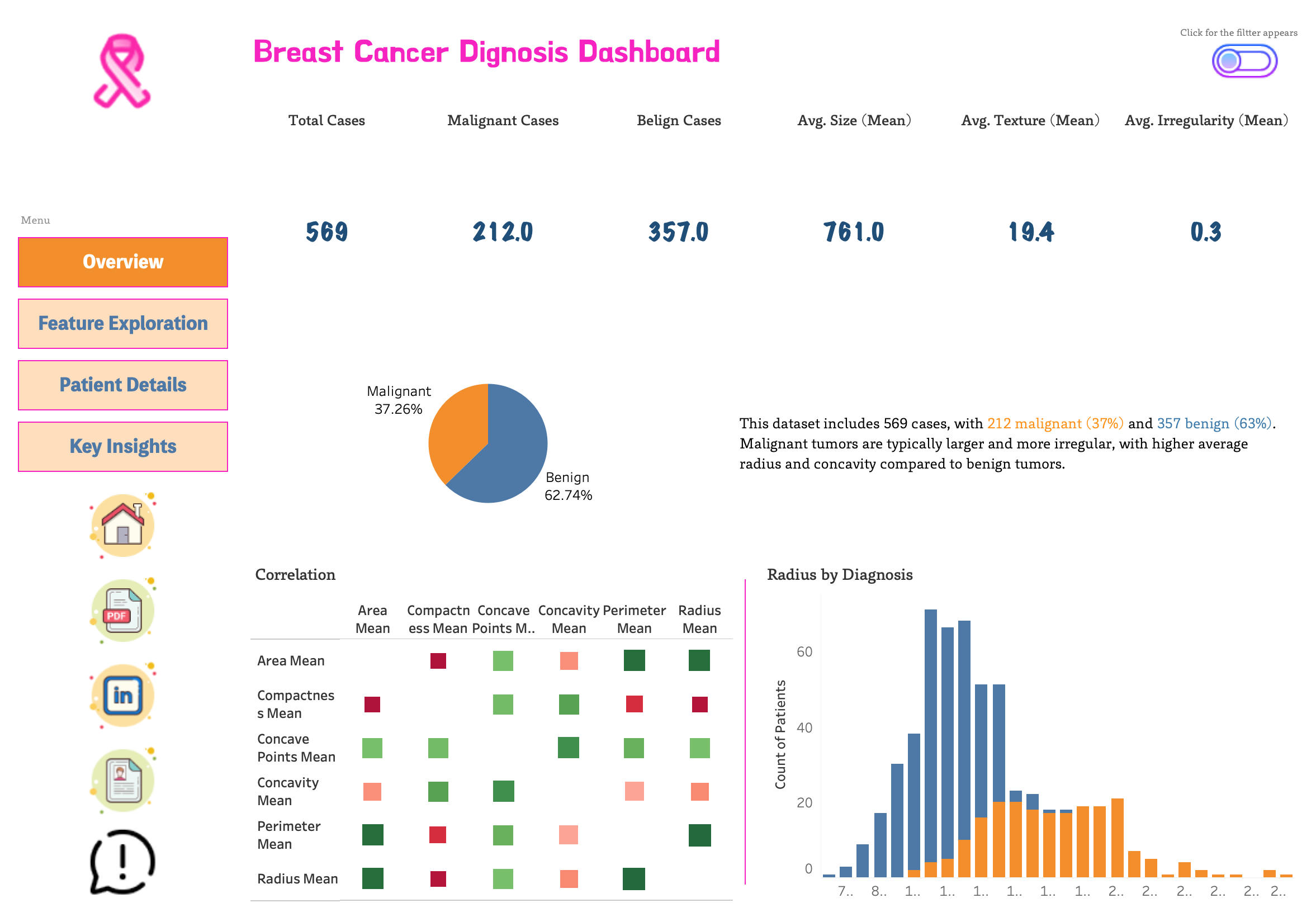
- Overview – KPIs, diagnosis distribution, mini correlation heatmap
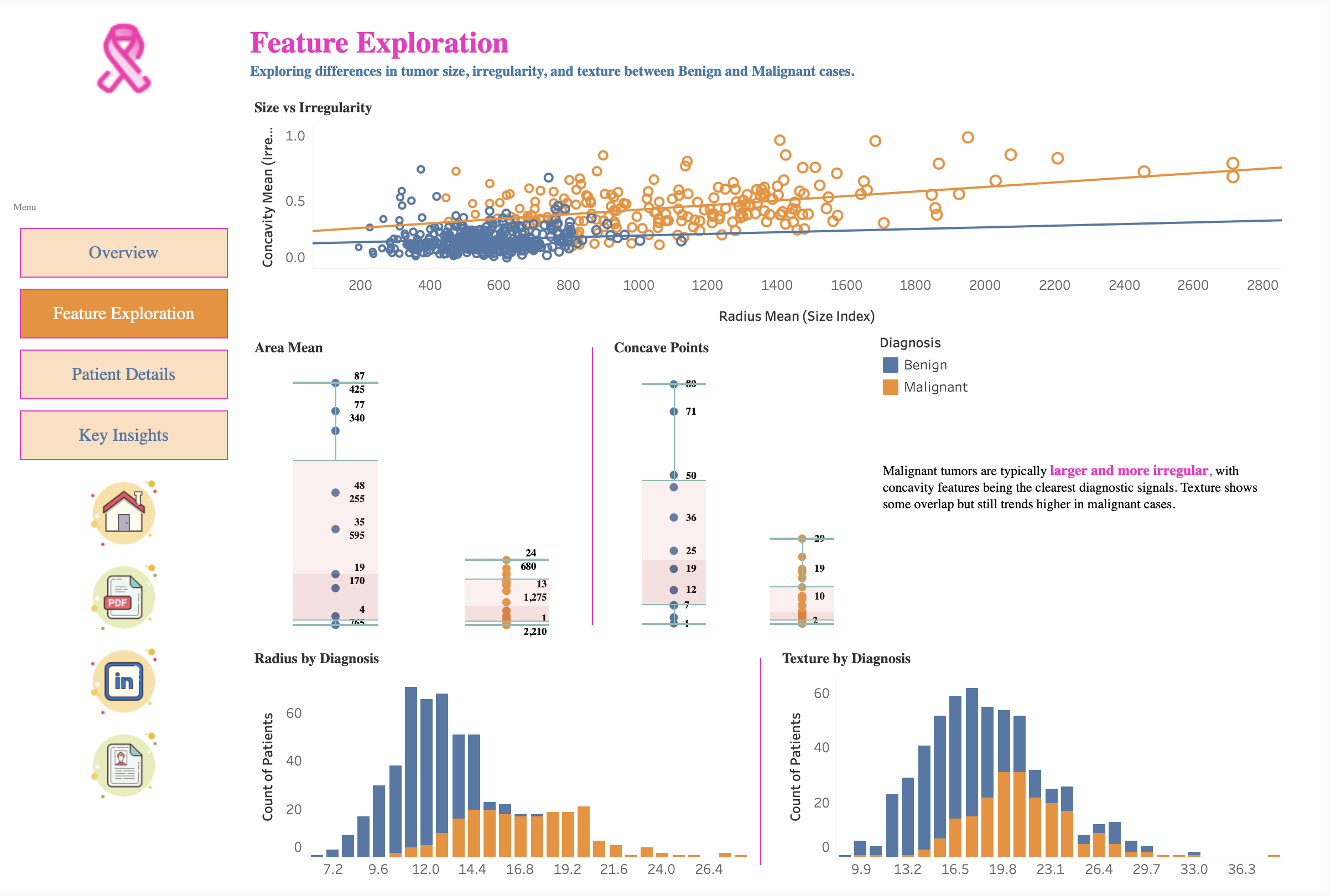
- Feature Exploration – scatter (size vs irregularity), box plots, histograms
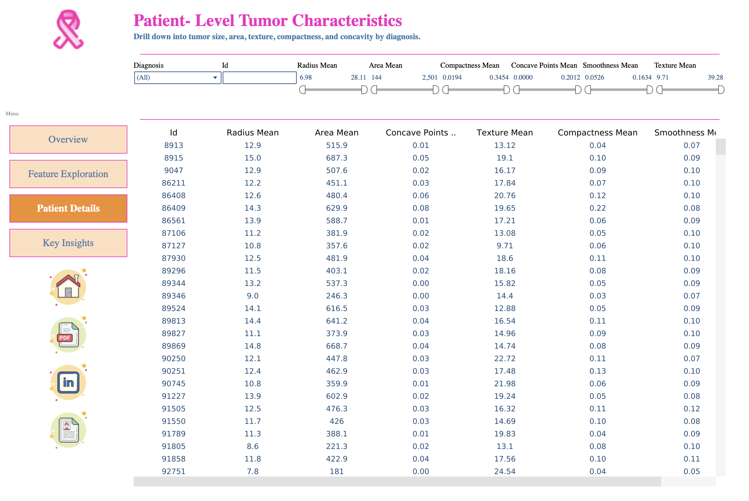
- Patient-Level Tumor Characteristics – filterable table (ID, diagnosis, key features)
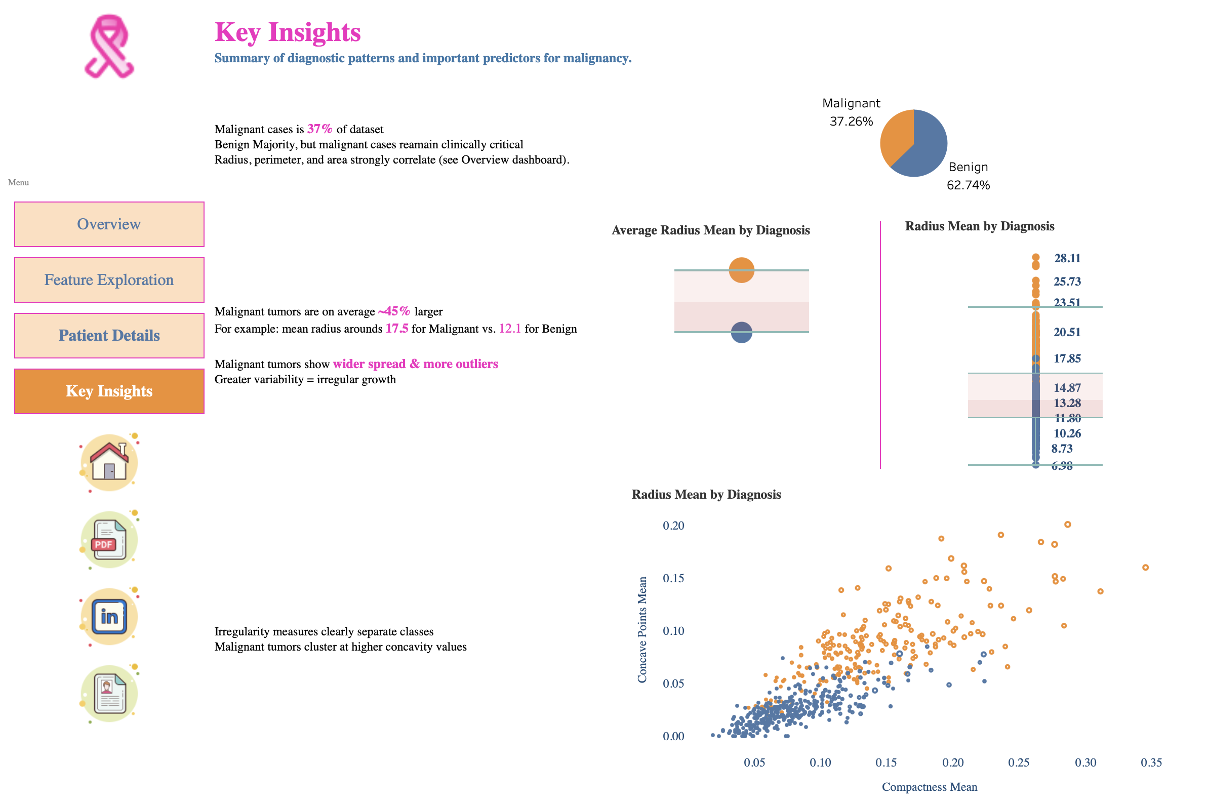
- Key Insights – one-page executive summary with annotated visuals
Key Insights
- Class balance: ~37% malignant / ~63% benign
- Size differences: malignant tumors are generally larger (e.g., radius, area)
- Variability: malignant shows greater spread (higher SD)
- Irregularity: concavity, compactness, concave points separate classes strongly
- Correlation: radius–perimeter–area are highly correlated (partly redundant)
Reproducibility
The 6-feature correlation heatmap is generated in Python and imported into Tableau:
- Run
notebooks/correlation_mini.ipynb(or a Colab notebook) to producedata/correlation_matrix_mini.csv. - In Tableau: connect to the CSV → build heatmap (Feature1 on Columns, Feature2 on Rows, Color = Correlation).
- All other visuals connect directly to the Kaggle dataset.